Should we predict covariates in an LSTM for timeseries forecasting?

1. Introduction

This blog accompanies a paper I wrote on the effect of covariates on LSTM networks for timeseries forecasting, which you can find on arxiv.

In business, leading indicators serve as vital signposts, offering insights into what the future may hold based on present measurements. For instance, the number of opportunities in a sales pipeline today provides a glimpse into future business closures. Similarly, during the pandemic, infection rates from tests were used to forecast future hospitalization rates. In the field of time series forecasting, where I spend a lot of my time, the integration of these leading indicators into our forecasting models would seem like an obvious choice. Not only should it enhance the accuracy of our predictions, but it should also enhances interpretability, enabling us to discern the driving factors behind our forecasts. This, in turn, would empower us to simulate various scenarios and potentially take actions to alter the future.

However, the reality is not as straightforward as it appears. Time series forecasting involves predicting the future based on past observations, with a long and well established history of traditional statistical models. In recent years, a plethora of deep learning models has emerged, offering improved forecasting capabilities over longer horizons and with more frequent data — a necessity in today’s world of IoT and big data. While many of these models support the inclusion of covariates, they typically assume that these covariates are known in the future. This poses a challenge when dealing with leading indicators that are only known in the present or past. One potential solution that was proposed by Salinas at al [1] in the DeepAR paper is to train the network to jointly learn both the target variable and the leading indicators, with the hope that it will leverage the latter to improve predictions. In this post we’ll explore this idea further by conducting a series of simple experiments to evaluate just how effective this approach is.

TL;DR: Our experiments show that for the most part, including covariates in an LSTM model does not improve forecasting performance. In some cases, it can even hinder performance. There are circumstances where our results show it can improve performance and given the somewhat artificial nature of our experiments, it’s possible that with more sophisticated models and feature engineering, covariates could be used to improve forecasting performance.

2. Methodology

I like to keep things simple. The simpler the better. So we’re not going to throw the kitchen sink at this problem to try and claw out a few percentage points of improvement. The aim here is to understand the fundamental behaviour of the network in the hope that we can gain some empirical insights that will guide us in future experiments.

So our here’s the plan: We will start by utilizing four publicly available datasets from the Monarsh repository, previously benchmarked against various models, including popular neural network architectures.

1. ‘hospital’: Consists of 767 monthly time series depicting patient counts related to medical products from January 2000 to December 2006
2. ‘tourism’: Monthly figures from 1311 tourism-related time series
3. ‘traffic weekly’: includes 862 weekly time series showing road occupancy rates on San Francisco Bay area freeways from 2015 to 2016
4. ‘electricity hourly’: Electricity dataset was used by Lai (LSTNet) and represents the hourly electricity consumption of 321 clients from 2012 to 2014

These datasets are univariates (ie they don’t have leading indicators) so we’re going to artificially generate some leading indicators. Is this representative of the real world? No, but it allows us to control a number of variables such as the levels of correlation and how many timestep into the future the leading indicators take effect. Our leading indicators will be generated based on the value of a target value at a given future timestep, to which we’ll add varying degrees of noise to control the correlation. We’ll run experiments for 1, 2 and 3 covariates where each additional covariates will be correlated with a target that is one additional timestep into the future. In otherwords, the first covariate will be correlated with the target at the next timestep, the second covariate will be correlated with the target at the timestep after that and so on. The network will have to learn that a given covariate is correlated with the target at a future timestep and use this information to improve predictions.

Next we’re going to need a model and in fact we’re going to use two models. Both share the same basic architecture. They are both autoregressive LSTM models that generate point predictions one step at a time. Again this is a really simple approach, but there is some relevance to this. Whilst Transformers have taken the world by storm, RNNs are still a popular choice for timeseries forecasting and since this approach of jointly training covariates and target variables was first proposed in the DeepAR paper, an autoregressive LSTM model, it seems fitting to use an RNN for our experiments.

Why two models? Well we’re going to use a base-lstm model as a baseline to compare our results against. This is going to reuse the majority of the conditions that the original benchmarks were run on, including the lookback window, but since we’re not going to allow ourselves the luxury of feature engineering lag variables like you get for free with GluonTS we don’t expect this model to perform as well over longer forecast horizons. In fact I was a bit concerned about what conclusions we might draw from this model if it performed poorly, so I decided to create a second model, the seg-lstm model. This model is identical to the base-lstm model with one exception. The input data is segmented into seasonal segments. This allows us to accomodate far greater context lengths (lookback windows) and therefore we hope should be better at predicting long forecasting horizons. As it turns out, the seg-lstm model performed much better than I expected.

3. Experiment Setup

For each dataset and model combination we’re going to run 30 experiments with the following scenarios:

1. 5 univariate scenarios with different seeds.
2. 8 scenarios with 1 covariate and different correlation (PCC) values
3. 8 scenarios with 2 covariates and different correlation (PCC) values
4. 8 scenarios with 3 covariates and different correlation (PCC) values
5. 1 scenario with 2 covariates positioned at t=1 and t=3 with a PCC of 1.0

The number of covariates will be denoted with the letter ‘k’. The correlation levels will be controlled to a range between 0.5 (strong positive correlation) and 1.0 (perfect correlation), In other words where k=1 and PCC=1.0 we will provide the model with a leading indicator that is the value of the target variable at the next timestep.

4. Results

In terms of the univariate benchmark results base-lstm yielded comparable results on the Hospital and Traffic datasets, slightly inferior results on Tourism, and significantly poorer results on Electricity. The seg-lstm model emerged as the top performer on Electricity with RMSE, whilst on Tourism it ranked second with MAE and RMSE. Overall, both of our models demonstrated comparable performance to the benchmarks on the shorter forecast horizons of Hospital and Traffic, while the seg-lstm model also displayed competitive performance on Tourism and Electricity.

Benchmark Univariate performance

Models	FFNN	DeepAR	N-Beats	Wavenet	Transformer	base-lstm	seg-lstm
Hospital (12)	18.33	17.45	17.77	17.55	20.08	17.52	18.05
Tourism (24)	20.11	18.35	20.42	18.92	19.75	21.50	19.85
Traffic (8)	12.73	13.22	12.40	13.30	15.28	12.77	12.97
Electricity (168)	23.06	20.96	23.39	-	24.18	34.12	21.20

Forecast horizons are given in the brackets.

To some extent the relative differences between the covariate and univariate cases are somewhat specific to the dataset. The models trained on Traffic appear to benefit the most from covariates giving improved results in the majority of cases. Conversely models performed worst on, Tourism only outperforming univariate in a few scenarios with perfectly correlated covariates.

Covariate vs Univariate performance

Models	covariates	base-lstm	base-lstm	seg-lstm	seg-lstm	seg-lstm	seg-lstm
correlation		1	0.9	0.5	1	0.9	0.5
Hospital (12)	k=0	17.52	17.52	17.52	18.05	18.05	18.05
	k=1	16.13	17.45	17.77	16.07	17.96	18.09
Tourism (24)	k=0	21.50	21.50	21.50	19.85	19.85	19.85
	k=1	20.54	22.17	28.18	19.14	20.32	21.56
Traffic (8)	k=0	12.77	12.77	12.77	12.97	12.97	12.97
	k=1	11.36	12.59	12.89	11.64	12.85	13.00
Electricity (168)	k=0	34.12	34.12	34.12	21.20	21.20	21.20
	k=1	33.10	30.41	33.95	21.01	22.37	21.45

Forecast horizons given in the brackets.

The effect of correlation on performance

We are interested in the performance of models in the special cases where the forecast horizon matches the number of covariates, as in these cases the model is effectively provided with information required to predict each timestep. Unsurprisingly the performance is best when the correlation is perfect to the extent that an almost perfect prediction was obtained in the cases of Traffic and Hospital. However the performance quickly falls away as the correlation weakens. Interestingly even in this highly artificial and advantageous setting, the error on Tourism and Electricity are still worse than the univariate case at correlation levels less than 0.9.

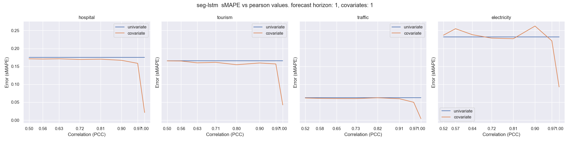
Fig 1. sMAPE error vs correlation

With the exception of Traffic, as the forecast horizon extends any performance advantage over a univariate setting diminishes for a corrrelation value of 0.9 and below when forecast horizon exceeds 3-4 timesteps. Looking at the differences between base-lstm and seg-lstm. We see that both models share common characteristics when examining the errors on forecast horizon trajectories. The stronger model in univariate scenarios will also perform better in a covariate setting.

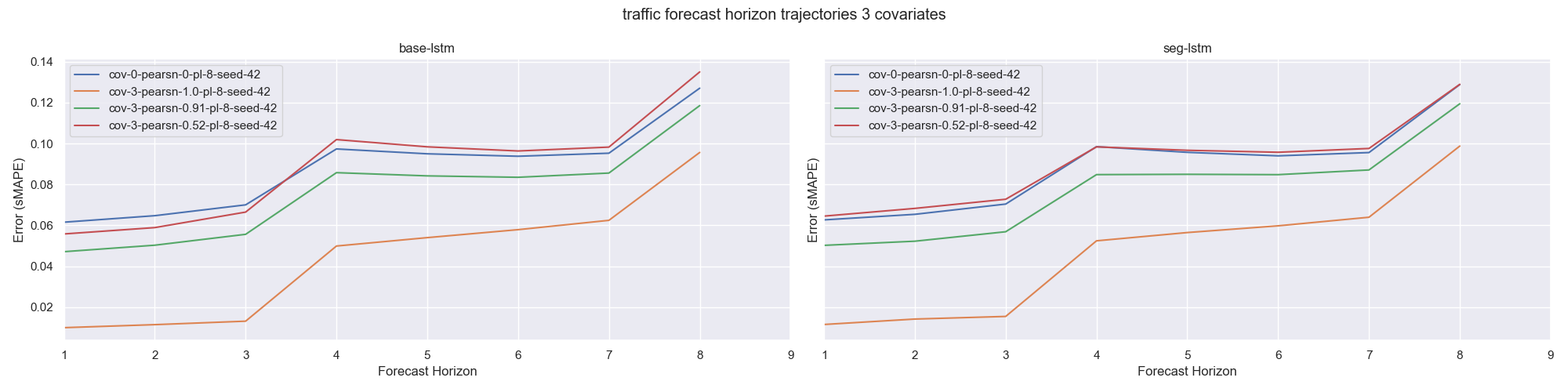
Fig 2. Traffic sMAPE error vs correlation with 3 covariates

The effect of multiple covariates on performance

Turning to comparing multiple covariates. Fig 3 shows sMAPE across full forecast horizons for 1, 2 and 3 covariates on the Hospital dataset with the special case of perfect correlation. Note that the error reduces as the number of covariates increases. Interestingly, on base-lstm the addition of each covariate shifts the onset of significant errors by one timestep. (i.e. errors start to accumulate at t=1 for k=1, at t=2 for k=2 and t=3 for k=3). It is conceivable that a model may be using covariate values from the current timestep alone rather than utilising covariates from previous timesteps. The network does not require covariates from previous timesteps in order to predict the subsequent 3 timesteps to produce the error improvement that we observe. Consequently we don’t know if the model is utilising covariates across the temporal dimension or if it is just using the current timestep’s covariates. One way to help answer this is to omit the second covariate meaning that at any given timestep the input contains lead indicators for values at t and t+2 and the model would have to obtain the leading covariate for t+1 from the input from the previous timestep. If the error trajectory in this example continues to exhibit the same 3 timestep offset that we observe with 3 covariates then we reason that the model must be learning across both temporal and feature dimensions simultaneously. It is evident from the plotted series, labelled as cov-2-pearsn-1.0-pl-8-seed-42-skip-1, that the error closely resembles that of using 3 covariates.

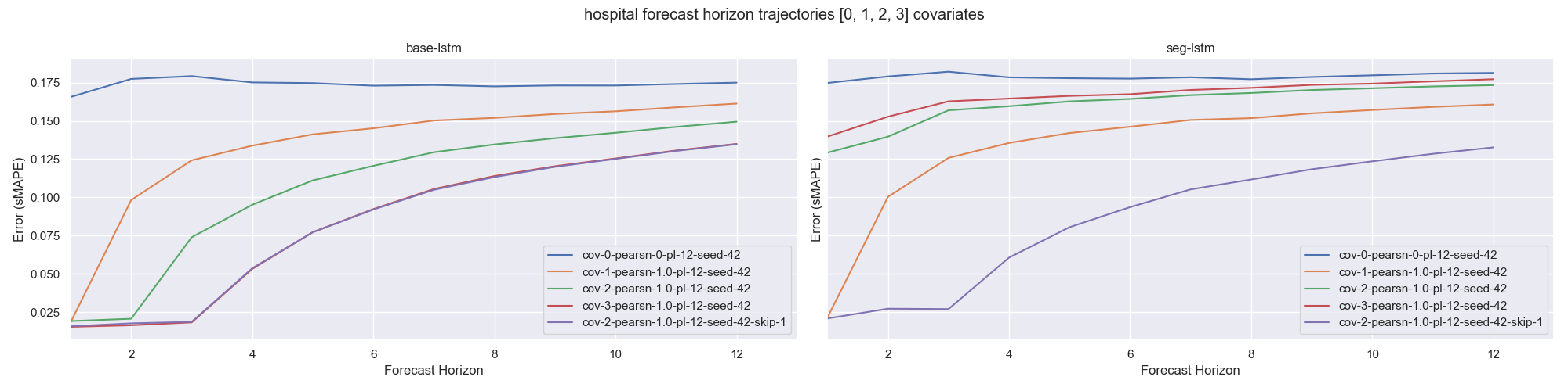
Fig 3. Hospital sMAPE Error with various covariates perfectly correlated

5. Conclusion

Given the aim of this study was to explore the effect of covariates on LSTM networks, it’s evident that predicting covariates jointly with target variables can under very limited conditions result in a performance improvement. As forecast horizons extend however, it frequently hinders performance. While acknowledging the artificial nature of the experiments used in this study it nonetheless underscores some potential for covariates to assist neural networks in making more accurate predictions.

It may be possible that the vanilla LSTM’s struggle to learn the relationships between covariates and target variables across long forecast horizons and that alternative architectures and/or additional feature engineering techniques

Future studies could also evaluate the use of covariates with more representative real-world data. Additionally, further exploration with artificial datasets could investigate the effects of other characteristics like extending the covariate lead time offset on target variables, non-stationarity or negative correlations. This raises the question of whether providing the network with information regarding the temporal influence of each leading indicator on the target variable could simplify the learning task.

The code for this study is available on my GitHub repository. Feel free to explore the data and models used in this study and to experiment with different configurations to gain a deeper understanding of the effects of covariates on LSTM networks. Github

References

1. DeepAR: Probabilistic Forecasting with Autoregressive Recurrent Networks