A fistful of MASE: Deconstructing DeepAR

1. Introduction

Hey Amigos! Four years since its release, DeepAR is an old timer in the world of neural networks for time series forecasting, but it can still outshoot many of the young guns out there and remains a popular choice to benchmark against. But like many gunslingers, it can be elusive and hard to pin down what makes it tick. In this post, we’re gonna get our hands dirty and deconstruct DeepAR to understand what really drives its performance. In particular we’re going to use the Pytorch GluonTS implementation as our reference. So saddle up and let’s get rolling.

2. The Good

DeepAR is not so much a model, but a complete system for time series forecasting and combines feature engineering, a model architecture and a probabilistic output that gives forecasts with prediction intervals (confidence intervals). I want to start our analysis with the core of the model, which is an auto-regressive LSTM. Before 2017, the way to model any type of sequence problem in a neural network was to use a recurrent neural network (RNN), due to their ability to use memory to retain information from earlier steps in the sequence. [Actually I just remembered that’s not quite true as Deepmind’s Wavenet was a CNN, but anyway I digress, you get the point]. The LSTM is a type of RNN that has a more sophisticated memory mechanism and is therefore able to capture longer term dependencies. Auto-regressive models use the output from the previous time step as input to the current time step, allowing the model to just babble away and generate sequences until someone tells it to stop.

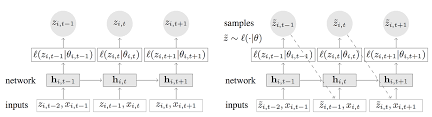
DeepAR Encoder-Decoder Architecture source

The model is described as having an encoder-decoder architecture, which at first glance can make it seem more complex than it really is. Typically, an encoder-decoder architecture takes some high dimensional input and compresses it into a lower dimensional “latent” representation and the decoder then takes this latent representation and generates a high dimensional output. There are a number of advantages to this, but one is that it allows the encoder and the decoder to have different architectures. In the case of DeepAR the encoder and the decoder are the same architecture, and not only that but they share the same weights. There seems to be a family resemblance, but they are not brother and sister, they are the same person, mathematically equivalent. The encoder and decoder are described separately probably to make it easier to understand the concepts in the paper. Once we take this into account, and if we ignore the output layer, what we’re left with is basically a bog-standard vanilla LSTM.

3. The Bad

So let’s talk about how this model generates forecasts. Like many models used for time-series forecasting DeepAR generates probabilistic forecasts, that is it generates samples from a distribution which enable us to calculate point averages and prediction intervals (confidence intervals). This gives our forecasts a measure of uncertainty, which is important in virtually all applications. So what DeepAR actually outputs for each data point are the parameters of a distribution. Every gun makes its own tune and there are many types of distributions, each one with its own characteristics defined by its own parameters. By default the GluonTS implementation uses a StudentT which looks like a classic bell curve and is parameterised by the mean and the degrees of freedom, which is akin to variance. Therefore, for every data point, DeepAR generates both a mean and a variance. These parameters allow us to define a distribution, from which we can subsequently sample during prediction. Typically we would sample from this distribution many times and then use this as the basis for our forecast. In the case of DeepAR, there’s an adjustment which is made to scale the values to the original scale which we’ll talk about later, but essentially this is how it works. Training the model is done by minimising the negative log likelihood of the distribution, or in English, we’re trying to make the model produce distributions that maximise the likelihood that the actual data comes from that distribution. So far so good. The problem starts when we want to evaluate the model performance using the GluonTS’s metric calculations for errors such as MASE, sMAPE, MAPE and MSE. In these cases we need point predictions, so typically we would take an average of our samples like the mean and calculate the error from that.

 def get_base_metrics(
        self,
        forecast: Forecast,
        pred_target,
        mean_fcst,
        median_fcst,
        seasonal_error,
    ) -> Dict[str, Union[float, str, None]]:
        return {
            "item_id": forecast.item_id,
            "forecast_start": forecast.start_date,
            "MSE": mse(pred_target, mean_fcst)
            if mean_fcst is not None
            else None,
            "abs_error": abs_error(pred_target, median_fcst),
            "abs_target_sum": abs_target_sum(pred_target),
            "abs_target_mean": abs_target_mean(pred_target),
            "seasonal_error": seasonal_error,
            "MASE": mase(pred_target, median_fcst, seasonal_error),
            "MAPE": mape(pred_target, median_fcst),
            "sMAPE": smape(pred_target, median_fcst),
        }

Backtest metric generation code from GluonTS source

But the mean is not the only way to calculate a point prediction, you could also use the median, or the mode. The mean is the most common, but it’s not always the best, and metrics such as MAE, MASE and MAPE are quite often better when calculated using the median, whereas MSE and RMSE are better with the mean. So the problem is GluonTS uses the mean to calculate MSE and the median to calculate MASE, MAPE and sMAPE for the same set of samples. It then presents these metrics as one set of results without any indication of which point prediction was used.

Well partner you only get to shoot those bullets once. You can’t put them back in the gun and have another go in the hope that you’ll get closer to the target and you can’t pick and choose which set of point predictions are used for which metrics. At the very least it should be clear which point prediction was used for which metric, or better still make two sets of results one based on the mean and one based on the median.

4. The Ugly

Let’s get into where DeepAR really gets its sharp shooting skills from. Now we start.

Scaling Neural networks work better when the inputs that we feed into them are in a range roughly between -1 and 1. A way to achieve this is to scale the entire dataset using standard normalisation which means that we subtract the mean and divide by the standard deviation. When we make predictions we perform the inverse operation to get the predictions back into the original scale. Sometimes I have seen this referred to as “global scaling”. DeepAR uses a different approach which you might think of as “local scaling”. The raw values of the dataset are fed into the model in mini-batches and for each mini-batch we perform a scaling operation, using mean absolute scaling, which means that each datapoint is divided by the mean of the absolute values of the mini-batch. We then need to store the scaling factors and perform the inverse operation at prediction time. With its distribution output you could do this directly on the samples, and there are certain distributions where this is necessary, but by default scaling is done by modifying the parameters of the distribution and then the samples that are generated are in the correct scale.

Covariates Another unique feature of DeepAR is the inclusion of some very specific covariates and this is where things start to get real ugly. I’ve discussed covariates in a previous post, essentially they are additional features that can help inform the network about the data in order to improve the forecast. Covariates may be static, meaning that they don’t change over time or time dependent meaning that they do. The paper makes reference to a “a single categorical item feature” which is a fancy way of saying that they have a static categorical feature which identifies the time series. In GluonTS you are required to provide a “unique_id” and in my opinion the intention was to use this as the categorical feature. However the code does not use this feature, and instead just sets a default value of 0 which is used to look up the embedding. In otherwords the feature contains the same value all the time and therefore carries no information.

The time dependent covariates are a little more interesting. The paper discusses an “Age” feature as being the distance to the first observation in that series. In GluonTS this is implemented using the following formula:

age = np.log10(2.0 + np.arange(length, dtype=self.dtype))

Age feature calculation in GluonTS source

In other words we number each item in the timeseries by it’s position in the sequence add 2 and then take the base 10 log. Now there are some implications of this that are not immediately obvious. Firstly, for this to work as intended any time we make a forecast we need to know the first observation of the entire series including all of the training data. Secondly, if there are multiple timeseries in the dataset with different start dates (as in the Tourism dataset) then the “Age” feature will be different for equivalent dates in different series. I know there are probably ways of working around this with padding values, but the principle of this feature instinctively feels wrong to me and a better and simpler approach would be to take the unix timestamp of each timestep scaled by some common factor.

The second time dependent covariate are the “time features” which are things like day of the week and the hour of the day. For a monthly dataset like the Tourism dataset, GluonTS implements just the month number and scales it using a max min scaler which forces the values to be in a range between -0.5 and 0.5. Again this feels wrong to me, and here’s the problem. When we plot this feature we see that it takes on this sawtooth shape, which has a minimum in January and a maximum in December.

Plot of the month feature

This is because January is month 1 and December is month 12. This means that we are telling the model that the months that are most dissimilar are January and December which in reality is not the case. A better approach would be to use something like the positional encoding schemes used in transformers which use a sine and cosine function to encode the position of the timestep with the wavelength set to the seasonality (ie 12 for monthly time series). This would give us a continuous representation where adjacent timesteps are more similar than distant timesteps.

Lastly we have a “scale” feature, which simply takes the log of the scale value calculated with the mean absolute scaling. I’m not entirely sure why this works, but my perception from using this on the base-lstm model from my last post, is that it does indeed help the model pick up the trend of the data more accurately. However I have no empirical proof of this in DeepAR so we’re gonna test that now.

So, my hypothesis is that none of these features in their current form actually help the model to make better forecasts. I’m going to test this by performing what’s called an ablation study. This means that we will train several models with different combinations of features and then compare the results. We train each model 5 times with different seeds and then calculate the average of the metrics for the tourism dataset and the electricity dataset. Now to be clear, we are going to use my implementation of DeepAR), which is not the same as the GluonTS implementation. My implementation produces point forecasts and is therefore trained as a regression task. Yes I know that DeepAR is a probabilistic model, but for the purposes of finding out which features are making a difference, I think we can safely ignore this. Apart from this the model architecture and the dataset are the same.

Electricity MASE

Tourism MASE

If you’re interested you can find more details on these WandB projects Electricity and Tourism, but to me with Electricity it looks like there maybe some suggestion that using few features is better than using many, but not statistically significant. The tourism results are all within the same standard error. My conclusion overall is that these features either individually or collectively do not help the model to make better forecasts.

So if we’re using a vanilla lstm and these covariates are not helping, what is it that makes DeepAR so good? Well, partner take a seat by the campfire and I’ll tell you.

When you create an estimator in GluonTS you can specify a lag sequence. This is a sequence of historical timesteps that will be added to each timestep as covariates. If we specify a lag sequence of 12, then alongside our input data we will also include the data from 12 timesteps ago ( or a year ago in the case of a monthly dataset like Tourism). If you don’t specify a lag sequence, then GluonTS will create one for you based on the frequency of the data. For a monthly dataset like Tourism the default lags are:

[1, 2, 3, 4, 5, 6, 7, 11, 12, 13, 23, 24, 25, 35, 36, 37]

Lag sequence for monthly dataset

For an hourly dataset like electricity the lag sequence contains 40 lags between 1 hour and 721. Now if you’re there thinking, isn’t it a bit odd that we’re using covariate features that contain temporal information from the past in a model whose architecture is designed to capture temporal information from the past, then you’re not alone. What impact do these lags have on performance, well let’s test it and find out. As before we’re going to train models with different lag sequences and compare the results. We’ll start off with 1 lag and gradually add more and more.

Tourism Lags MASE

What do you think of that? The more lags we add the better the model performs. My boy, you’ve become rich. It seems we’ve found the secret sauce that makes DeepAR so good.

5. Conclusion

One of the key issues that I think we have with the benchmarking of these models is the size of the context length or the look back window. This is how many timesteps the model can see in the past when we use recurrence. For Tourism it’s 15 and Electricity it’s 30. Let’s just put that into perspective, we’re going to provide a day and a quarter of data to a model and expect it to forecast the next 7 days. Now I’m not saying that if the context lengths included the same time range as the lags that we could exclude the lags and still get the same performance but I do think that this configuration does not allow the lstm to do what it does best.

Overall, despite my misgivings about the covariates and some of the implementation details, DeepAR is a very powerful model that can outperform even the latest generation of transformer based models and maybe there are some areas where it can be improved further still.

So there you have it, a look at what makes DeepAR tick and this is where we part ways, so long, adios amigos.