
Revisiting Playing Atari with Deep Reinforcement Learning
It's been over a decade since Mnih et al. published their groundbreaking paper, marking the first successful fusion of reinforcement learning and deep learning. This seminal work introduced the Deep Q-Network (DQN) and set the stage for subsequent research, ultimately giving rise to innovations like AlphaGo, AlphaStar, and more.
What makes this paper extraordinary is its simplicity – it merely requires pixel values from an Atari emulator as input. There are no game-specific features provided; the agent learns solely from what it can "see" on the screen. This flexibility allowed the authors to use the same architecture and hyperparameters to train agents for a variety of Atari games.
Motivated by this pioneering work, I embarked on a journey to revisit the original paper and its 2015 Nature follow-up. My goal was to recreate the results using PyTorch, gaining a deeper understanding of the field. Specifically, I challenged myself to train a DQN on Breakout until it reached human-level performance, mastering the optimal strategy described in the Nature 2015 paper:
“Breakout: the agent learns the optimal strategy, which is to first dig a tunnel around the side of the wall, allowing the ball to be sent around the back to destroy a large number of blocks.”
Oh and there's one last catch - we're going to do this on a single GPU hosted on Paperspace Gradient in a single session (approximately 6 hours).
To achieve this, we'll use a Jupyter notebook, an Atari emulator from Gymnasium, and PyTorch. We'll also log our results to Weights & Biases to track our progress. The complete code is available on GitHub
1 Deep Reinforcement Learning
The 2013 paper's contributions are pivotal, focusing on using a Convolutional Neural Network (CNN) to directly learn Q values from images and introducing experience replay. Experience replay serves as a cache of historical memories (transitions) that the agent had with the environment. Each transition includes the state, action, reward, and new state.
In Q learning, the agent typically updates its Q values using the most recent transition. However, using a neural network to approximate Q values as the agent moves through the environment generally doesn't work in practice. Experience replay makes it possible to separate the process of generating data by the agent interacting with the environment and optimising the network by sampling historical memories from experience replay.
The complete algorithm for Deep Q-Learning with experience replay is as follows:
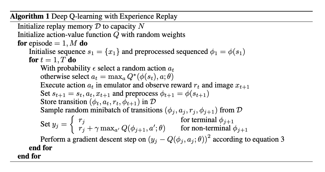
Figure 1. DQN with Experience Replay Algorithm
I find it easier to think about how the algorithm can be arranged in code. The following is a high-level overview of the implementation:
Data generation:
- Start a new game and observe the initial screen
- Preprocess the image and stack it with the previous 3 frames
- Select an action using an epsilon-greedy policy from the Q network
- Execute the action in the emulator and observe the reward and new screen
- Preprocess the new screen and stack it with the previous 3 frames
- Store the transition in the experience replay
Training:
- Sample a batch of transitions from the experience replay
- Compute the loss by comparing our current estimate of the Q values in the current state with the estimated Q values in the next state plus the reward
- Update the Q network parameters using gradient descent
Our experience replay is a simple Python deque with the ability to sample a batch of transitions.
Fig 2: Experience Replay implementation
Interestingly there's no target network as this concept was introduced in the 2015 follow-up and may well make our training unstable. We'll revisit this later.
2 Preprocessing and Model Architecture
The emulator that we work with provides us with the raw pixels from the screen. However, they were considered high resolution and to train a network on such a set of images would be computationally demanding therefore the paper describes a set of preprocessing steps that reduce the resolution and remove any unnecessary information before passing into the network.
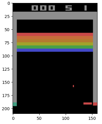
Figure 3. Raw image from the emulator
Original Size: 210 x 160 x 3
Greyscale: Combining RGB channels into one (210 x 160 x 1) Images come out of the emulator in RGB, and each colour has its own set of values called channels. Greyscaling combines the 3 colour channels into 1 (effectively making it black and white). Greyscaled size 210 x 160 x 1
Downsampling: Reducing resolution using interpolation (110 x 84 x 1) The images can be reduced further in size by reducing the resolution using interpolation. It is a technique that estimates the values of pixels at coordinates by considering the weighted average of the nearest four pixels. Downsampled size = 110 x 84 x 1
Cropping: Removing top and bottom regions not used in gameplay (84 x 84 x 1) The top and the bottom of the image can be removed since that part of the screen is not used in the playing area and therefore doesn’t contain any useful information that the agent can learn. Cropped size = 84 x 84 x 1
Stacking: Successive frames are stacked into groups of 4 (84 x 84 x 4) An issue considered was that there is no temporal information in an individual frame ( ie you don’t know which way the ball is moving or how fast), and to address that the input will actually consist of 4 conecutive images. It’s a bit like using the live setting on a phone photo in that you get a hint of movement.

Figure 4. Processed input to the network
Model Architecture: The model is surprisingly small even by the standards of the day with just 2 conv layers plus ReLU activations, a single FC layer with ReLU, and an output layer. Separating the logic for action selection from Q-value learning allows for easier adaptation of the CNN, as seen in the 2015 update.
Fig 5: Pytorch implementation of the 2013 conv net
Fig 6: DQN action selection logic
3 Experiments
Before running training, considerations include:
- DeepMind trained on 10 million frames, but due to time constraints, we aim for approximately 6 million frames.
- The experience replay stores 1 million transitions, but memory limitations necessitate reducing this to 450K.
- They used an RMSProp optimizer, however decided to use an Adam optimizer with a lower learning rate as detailed in the Rainbow paper.
- Early experiments suggested that terminating the episode after losing a life was beneficial. It's unclear if this is an approach that was used in the original paper. However in the 2017 Rainbow paper, the authors mention that they used this approach for Breakout.
- We also use reward clipping meaning that we either get a reward of 1 or 0. My initial implementation omitted this but I later discovered that the bricks higher up are worth more points and interestingly it looked like the agent was exploiting this by choosing to target bricks higher up.
- We will adopt the same epsilon annealing schedule and linearly anneal epsilon from 1 to 0.1 over the first million frames and then keep it constant at 0.1 for the remainder of training.
- The emulator that was used in the paper sends images at 60 fps, but they only used every 4th image effectively reducing the frame rate was reduced to 15 fps and to repeat the action taken for every frame that was skipped. Gymnasium emulator does this for us so our implementation does not include this.
The model was trained on a Free-A4000 instance on Paperspace Gradient for a complete 6 hour session.
4 Training and Stability
Now I must admit that I was highly sceptical that the model would converge at all. I had previously tried to train the much simpler CartPole environment using just DQN + Experience Replay with no success. However to my surprise the model training was remarkebly stable and after around 10 epochs the loss steadily decreeased. The profile of the validation reward also took a similar shape, although the average reward was much lower than the published results.
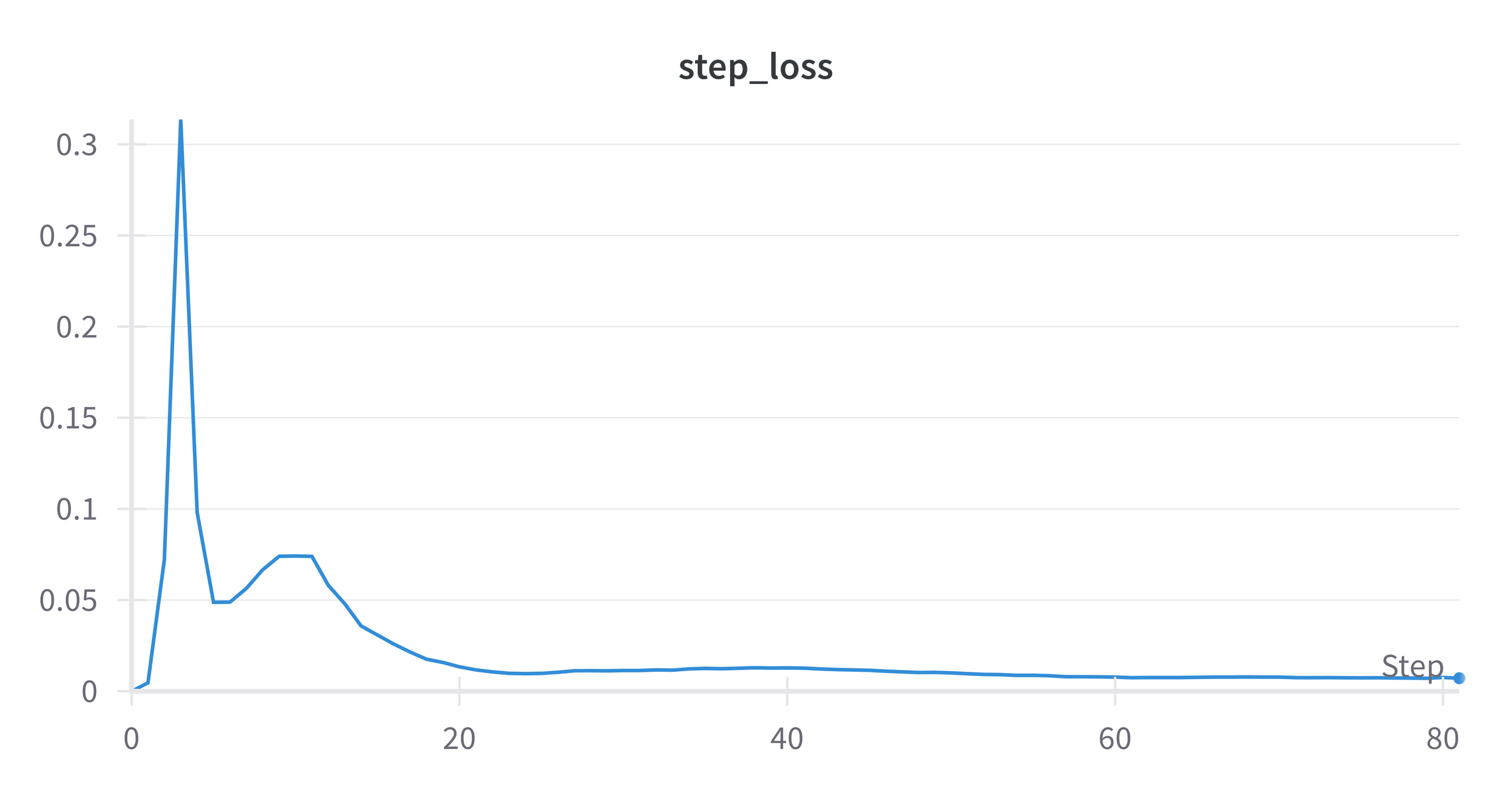
Figure 7. Step Loss
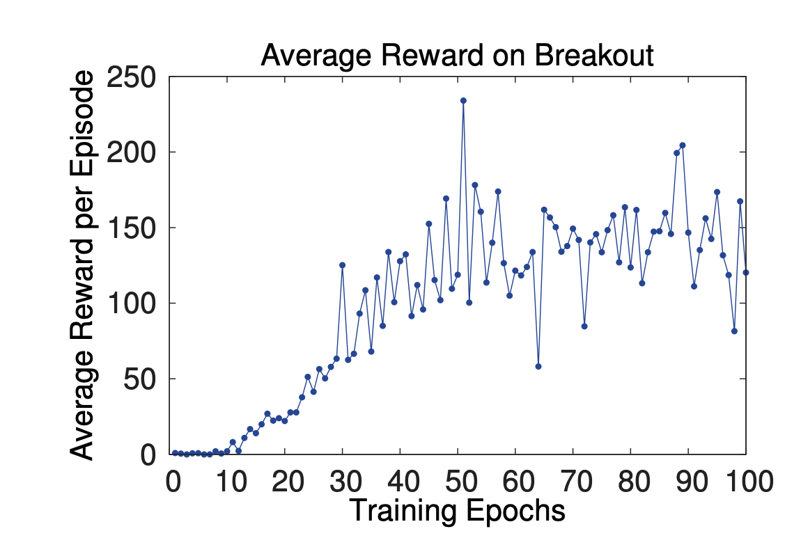
Figure 8. Deepmind reward

Figure 9. Our reward
5 Main Evaluation
The average validation reward for our model on the last epoch was 16 compared to the published score of 168. Assuming these are unclipped scores across an entire episode of 5 lives, it provides a benchmark for comparison. So what's the difference between our model and the Deepmind model? I suspect that the main difference is the experience replay size 1M vs 400K in ours. I suspect that had we increased the capacity of the experience replay then we would have seen a higher score, however the GPU memory was pretty much maxed out which would meant putting it in CPU memory which would have slowed down the training considerably. Overall the results are nowhere near what was published but it's still better than the alternatives at the time, and honestly I'm surprised that it worked as well as it did and we'll follow up with some improvements in the next post as we look at the 2015 Nature paper.
| Model | Average Score |
|---|---|
| Deepmind | 168 |
| Ours | 16 |
And in case you're wondering, here's what an agent with a score of 16 looks like: