LTSF-Linear: Embarrassingly simple time series forecasting models

You know in a world where there are more transformers in machine learning research than there are in my son’s bedroom, it was a breath of fresh air when I read the 2022 paper Are Transformers Effective for Time Series Forecasting by Zeng et al. They suggest that it’s possible to achieve comparable performance to state of the art transformers like Autoformer, Informer and Fedformer by using what the authors describe as embarrassingly simple linear models. Now this struck a chord with me partly because my relationship with transformers has been patchy to say the least and partly because being a simple kinda guy I liked the idea of simple models going head to head with the heavy weights in a David vs Goliath stand off. This post is going to take a dive into the paper, the models it introduces and we’ll see how they perform in the real world. All the code for this post can be found on my nnts github repo.

Transformers and Long Term Time Series Forecasting (LTSF)

So the paper doesn’t waste any time and from the off the authors essentially argue that the requirement for transformers to learn ordering through positional encoding puts it at a disadvantage because of the fact that inevitably some ordering information will be lost. They claim that this is not such a big problem in NLP because there is more to natural language than the precise ordering of words, but in time-series this is not the case.

So what the authors are referring to is the fact that a transformer architecture does not intrinsically understand the temporal relationships between the data points in a time series. This is because the transformer architecture is designed to learn the relationships between the tokens in a set and not the relationships between the positions of the tokens. This is why we need to add positional encoding to the input data to give the model some idea of the order of the tokens.

Instictively this point of view makes sense to me, but I would maybe go further. I think transformers are really well suited to learning abstract concepts, such as language and vision and that is why excel in those fields. However, in time-series and tabular data the statistical properties that we need to make predictions or forecasts are in plain sight.

It’s worth bearing in mind that when this paper was written the time-series Transformers were dominated by the “formers” family, like Informer and Autoformer, which were designed to address long forecast horizons on multivariate time series. Consequently the authors focus on comparing their models primarily in this domain although they do present some univariate results which we’ll come to later.

They propose 3 models called called Linear, NLinear and DLinear which all come under the family name of LTSF-Linear. They are all single layer linear models with no non-linear activation functions. These models are designed to be simple and useful for benchmarking, but still competitive with the state of the art transformers at the time of writing.

Model Architecture

These models share some common characteristics: the input is a time series of historical values and the output is a vector of future values whose length is the forecast horizon ( see figure 1 for an illustration of this). This is referred to as Direct Multi-step forecasting (DMS) and is in contrast to an auto-regressive model like DeepAR which predicts one step ahead recursively. Now with there being just one linear layer and no non-linear activation functions the model is linear and hence the names DLinear and NLinear. In otherwords there’s no deep learning going on here. There’s also no proabalistic output so the experiments in the paper optimise the models as a regression task using the Mean Squared Error (MSE) loss function. I guess technically speaking this makes them a linear regression model.

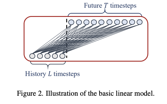
Figure 1 Linear Model Architecture showing Direct Multi-step (DMS) Forecasting

DLinear

DLinear handles the input by splitting it into 2 components. The first component is the trend and is determined by calculating the rolling average of the time series using a moving window defined by a hyperparameter kernel size. This is then subtracted from the original timeseries to give the second component which the authors refer to as the seasonal. The two components are then each passed through a linear layer to project them onto the forecasting output space and then summed to give the final output.

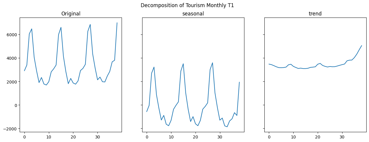
Figure 2 DLinear decomposition of Tourism Monthly

To illustrate what this means in practice figure 2 shows the decomposition of the first series in the Tourism Monthly dataset. The plots shows, from left to right, the original time series, the seasonal component, and the trend component. Note that the seasonal component is closely centered around zero and the trend component sets the initial value and the slope over time. By separating out these components we can now project each one in isolation into the future, the theory being that it is simpler to model the trend and the seasonality separately than it is to model the signal as a single thing.

If this sounds strangely familiar then you’re right to think that this is not the first time this idea has been tried. Indeed decomposing a time series into separate components has been around for hundred years or so and is the basis of the well known Holt-Winters statistical model.

NLinear

If you think DLinear is simple then NLinear takes things to the next level. It subtracts the value of the most recent observation from the time series, which effectively scales the observation and then passes this through a single fully connected linear layer to project it onto the forecasting output space. The most recent observation is then added back to the output to give the final forecast. That’s it, literally that’s the model!

Multivariate vs Univariate

Now I mentioned earlier that these are primarily multivariate models and that the authors present some univariate results. So before we go any further and discuss their experimental setup let’s just clarify what we mean by multivariate and univariate time series forecasting.

Most time-series forecasting datasets will comprise of a single file containing multiple time series. For example the Tourism Monthly dataset has 366 individual time series, one for each region in Australia, New Zealand and Hong Kong. Each time series is a sequence of monthly observations and the number of observations in each series may be different as the historical data may start at different times in each region. When we forecast we aim to predict the future values for each of the time series across a forecast horizon, but because the time series in the dataset do not necessarily share a common time span (eg one region may have started collecting data later than another) we do not attempt to model the relationships between each time series, so we forecast each time series individually of the others. This is what we refer to as Univariate. Our input is a single time series and our output is a single time series.

By contrast Multivariate forecasting is where we have multiple timeseries that do share a common time span and we aim to model the association between the time series. This means that the input to the model is essentially a table of values containing a sequence of historical values for each time series in the dataset. Obviously this requires the dataset to be structured in such a way that all the time series are aligned. Examples include ETTh, Electricity, Traffic and Weather datasets and these have almost become the de-facto standard for benchmarking long horizon multivariate time series forecasting models such as Informer and Autoformer. If knowing the temperature of a transformer at two o’clock next Tuesday is important to you then these are the models for you, but in my opinion they are not representative of the majority of time series forecasting problems.

In summary not all datasets are suitable for multivariate forecasting, but all datasets are suitable for univariate forecasting.

Experimental Setup

The models can be configured to operate in a channel dependent multivariate mode or a channel individual univariate mode. The input into the model always take the form of a table (matrix) with dimensions (L, C) where L is the Lookback window length of historical observations and C is the number of time series in the dataset.

Channel Dependent

In this configuration, we take our input as one lump and pass it through the the linear layers. In DLinear there are two ( one seasonal and one trend), and in NLinear there is just one. So effectively we are producing forecasts for all the “channels” in the dataset simulataneously with one or two big matrix multiplications. Computationally this is very efficient which is something that the authors highlight in the paper as a key advantage of these models in comparison to transformers.

Channel Individual

The channel individual mode is presented as somewhat equivalent to a univariate model. In this configuration a set of linear layers are created for each time series in the dataset. The weights of these layers are dedicated to one time series and are not shared. The univariate results are conducted using the ETT dataset, which has 7 time series, and following the same methodology as many of the transformer papers which uses just one time series from the dataset to train and evaluate the model. That is to say one time series is selected (in this case the “OT” feature), all of the other series are discarded and the model is trained and evaluated on this one time series. Now I have an issue with this approach because in my view this makes the model equivalent to a local model (ie a model that is trained for one time series in contrast to global being a single model trained to forecast multiple time series). As such I don’t think the results are directly comparable to global univariate models like N-HITS, DeepAR, and N-BEATS. Oh and by the way the authors are not the only offenders here, the same methodology has been used in many of the multivariate transformer papers.

As a side note there is no evidence in the paper that the channel individual configuration has been tested on a dataset with more than one time series, and I think had they done so they would have realised that it’s not such a great idea, because handling each time series individually with lots of tiny matrix multiplications is a real drag on performance and is a major problem for datasets that have a large number of time series. I will discuss this further in a future post.

Performance

So how do these models perform? We’re going to take a look at the results from the paper with the datasets that they use and then we’re going to take a look at how they perform on some of the datasets from the Monash benchmarks and compare them to the best performing models from those benchmarks.

Paper Results

So first I’ve implemented the code for the DLinear and NLinear models and their data sampling strategy. I’ve the run some experiments on the ETTh datasets in both univariate and multivariate configurations with a forecast horizon of 336 timesteps. The MAE metrics are shown in table 1 with our results shown in brackets next to the paper’s published results.

Model	DLinear Multivariate	DLinear Univariate	NLinear Multivariate	NLinear Univariate
ETTh1 (336)	0.443 (0.439)	0.244 (0.235)	0.427 (0.429)	0.226 (0.226)
ETTh2 (336)	0.465 (0.480)	0.367 (0.369)	0.400 (0.423)	0.355 (0.356)
ETTm1 (336)	0.386	0.182	0.388	0.172
ETTm2 (336)	0.342	0.261	0.327	0.259

*Table 1 MAE results for ETT dataset with a forecast horizon of 336 timesteps from the paper, our results are shown in brackets.

So, generally speaking we are able to do a pretty good job of reproducing the results from the paper, the one exception being the multivariate configuration on the ETTh2 dataset where we see a slightly worse result. In the paper the results are more complete and show that DLinear or NLinear outperform Autoformer, FEDFormer, Informer, Pyraformer, and LogTrans models.

Monash Benchmarks

So far so good, we have 2 models and are confident that we can reproduce the results from the paper. Now let’s see how they perform on some of the datasets from the Monash benchmarks. I’ve selected 6 multivariate datasets from the Monash benchmarks and we’re only going to measure the performance of the Multivariate configuration, because as we’ve discussed the univariate configuration isn’t really comparable.

Dataset	DLinear	NLinear	Autoformer	PatchTST	Informer	FFNN	DeepAR	N-BEATS	WaveNet	Transformer	Prophet
Carparts	0.752	1.045	1.247	1.075		0.747	0.747	2.836	0.754	0.746	0.876
COVID	5.601	5.176	7.221	8.111		5.459	6.895	5.858	7.835	8.941	12.77
Electricity Hourly	1.880	1.882	2.400	2.138	2.682	3.2	2.516	1.968	1.606	2.522	2.05
Electricity Weekly	0.780	0.792	0.929	0.846	1.444	0.769	1.005	0.800	1.250	1.770	0.924
Traffic Hourly	0.923	0.918		0.896	1.439	0.892	0.825	1.100	1.066	0.821	1.316
Traffic Weekly	1.096	1.103	1.476	1.168	1.323	1.150	1.182	1.094	1.233	1.555	1.084

*Table 3 DLinear and NLinear MASE compared to various other models. PatchTST and Autoformer results have been produced on the nnts framework. Informer, FFNN, DeepAR and N-BEATS and WaveNet results are all taken directly from the Monash benchmark figures. The best error is shown in bold.

So NLinear is the best model on the COVID dataset, and I think it’s fair to say that it compares well with the other multivariate transformer models, but can we really say they outshine the competition? Not really no.

Conclusion

So there we have it a look at the LTSF Linear models and how they perform in different scenarios. I think the authors claim that these models are competitive with state of the art multivariate transformers is justified. But the elephant in the room here is that with small to medium forecast horizons none of these multivariate models are really any better than univariate models and in most cases they are worse. Now it maybe that when you start using long forecast horizons (say in excees of 336 time steps), these models start to come into their own, but for anything shorter the question is: is it really worth it? And in my opinion probably not, but hey what would I know.. I’m just a simple guy trying to avoid treading on transformers in my son’s bedroom.

In the next post we’ll take a closer looks at channel individual / dependent configurations and see some very interesting results.