State of the art timeseries forecasting with 1Cycle scheduling

1. Introduction

In this, a follow up to my two previous posts DeepAR and superconvergence, I will show you how to obtain state of the art performance using my simplified version of the DeepAR model trained with 1Cycle scheduling on a selection of the Monash datasets.

2. Recovering lost performance

In the experiments that I ran for the DeepAR article, I created a version of DeepAR on my nnts repo. Now because I’m lazy and it was easier to implement, this version made point predictions, had some small differences in features and a simpler data sampling strategy. While it identified lag features as the biggest contributors to performance, it didn’t quite achieve the same results as the GluonTS DeepAR model, and this bothered me. So being a sucker for punishment I set about identifying where this last bit of performance could be coming from and after a long process of elimination I eventually came to the somewhat depressing conclusion that the biggest contributing factor was most likely the probabilistic head. Once I accepted that, I created a version of DeepAR with the same outputs as the GluonTS version that generates the parameters of a StudentT distribution. Now if I include the additional features that were previously omitted, and use a similar data sampling strategy which iteratively samples a window from each time series in the dataset we get the following results:

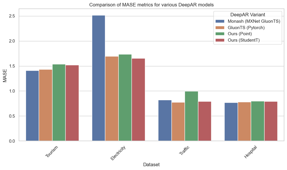
Figure 1. Comparison of MASE metrics for various DeepAR models

Dataset	Monash (MXNet GluonTS)	GluonTS (Pytorch)	Ours (Point)	Ours (StudentT)
Tourism	1.409	1.432	1.538	1.523
Electricity	2.516	1.697	1.737	1.656
Traffic	0.825	0.774	0.999	0.792
Hospital	0.769	0.784	0.799	0.794

Table 1. Comparison of MASE metrics for various DeepAR models

So going with the adage that 4 sets of results are better than 1 we have the following: Monash (MXNet GluonTS) are the results published Monash. These experiments were performed on the MXNet version of DeepAR from GluonTS. They also define the hyperparameters, context length and forecast horizons that we will use in all our experiments to keep things comparable. GluonTS (Pytorch) are tests that I have performed on the Pytorch version of DeepAR using GluonTS. With these small datasets there tends to be a lot of variation in performance, so I run all my experiments 5 times with different seeds and present the mean. Point DeepAR is my implementation of DeepAR trained as a regression task with a L1 Loss objective. StudentT DeepAR is my implementation of DeepAR with, unsurprisingly, a StudentT distribution probabilistic head. The test metrics are calculated using the median value from 100 samples drawn from the model. My models also use the GluonTS like data sampling strategy and the same covariate features. After all that, here’s the important bit, you should be able to convince yourself that the StudentT DeepAR model has a comparable level of performance to the GluonTS DeepAR.

3. Improving DeepAR

Having got a model that has comparable performance, I wanted to see if it would be possible to make it even better. I mentioned in my DeepAR appraisal that I thought it might be possible to improve the performance by making some modifications to how the age and date covariates are engineered. Well I tried various ideas: using a cyclical sine function to represent months, using an age feature that is based on the timestamp instead of the the length of the timeseries, and using embeddings for various date features, however none of these things seemed to really help. In the end I concluded that they did not make a difference and in fact just reinforced my previous results which suggested that the only features that really make a difference are the lag variables. So from here on the experiments use only lag variables and every other covariate feature is omitted.

4. 1Cycle to the rescue

So by now, I was starting to believe that maybe it’s not possible to improve performance, but I had a couple more ideas that I thought would be worth trying. One thing that I found which did make a difference was to tweak the scaling function that we discussed in the DeepAR post. I concluded the original mean absolute scaling function would not handle zero values well, because the scale would be close to zero and so the forecasted results would also be close to zero when we unscale them.

If you’ve read my previous post on super-convergence you will know that I am a big fan of 1Cycle scheduling and find that I get better generalisation with test set performance and more consistent results with less variation with different seeds. So I thought it would be worth trying here. I set the maximum learning rate to be 3x my original learning rate and ran the experiments with everything else the same. So I was very interested to see the results:

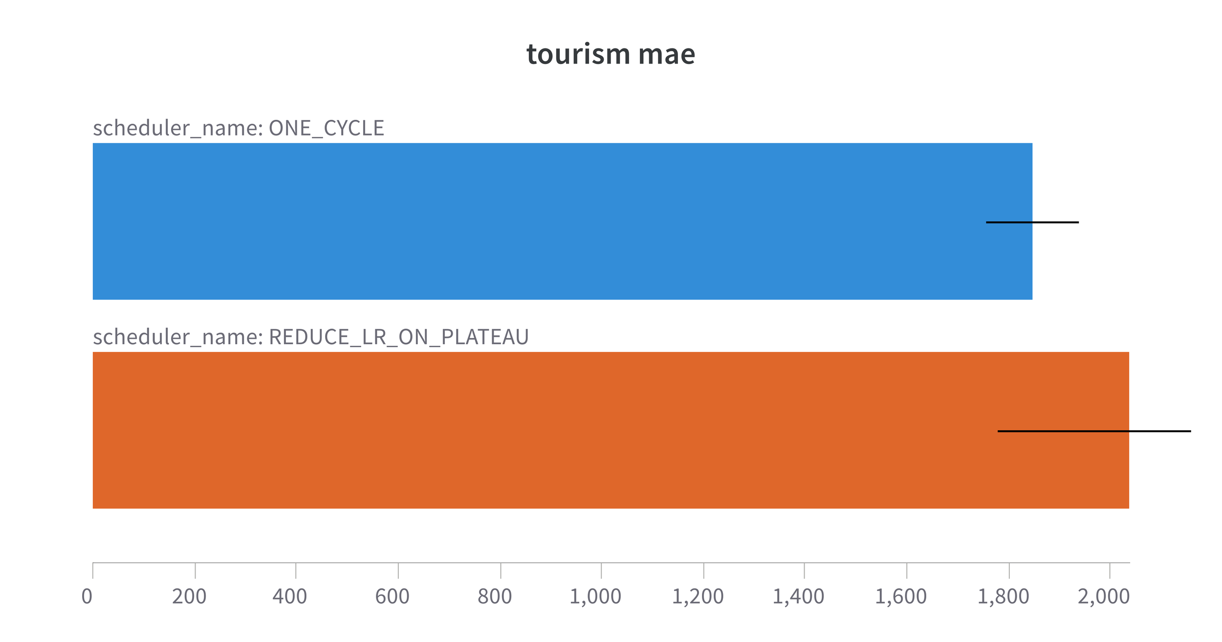
Figure 2. 1Cycle MAE with our model on the Monash Tourism monthly dataset. Forecast Horizon = 24 steps wandb

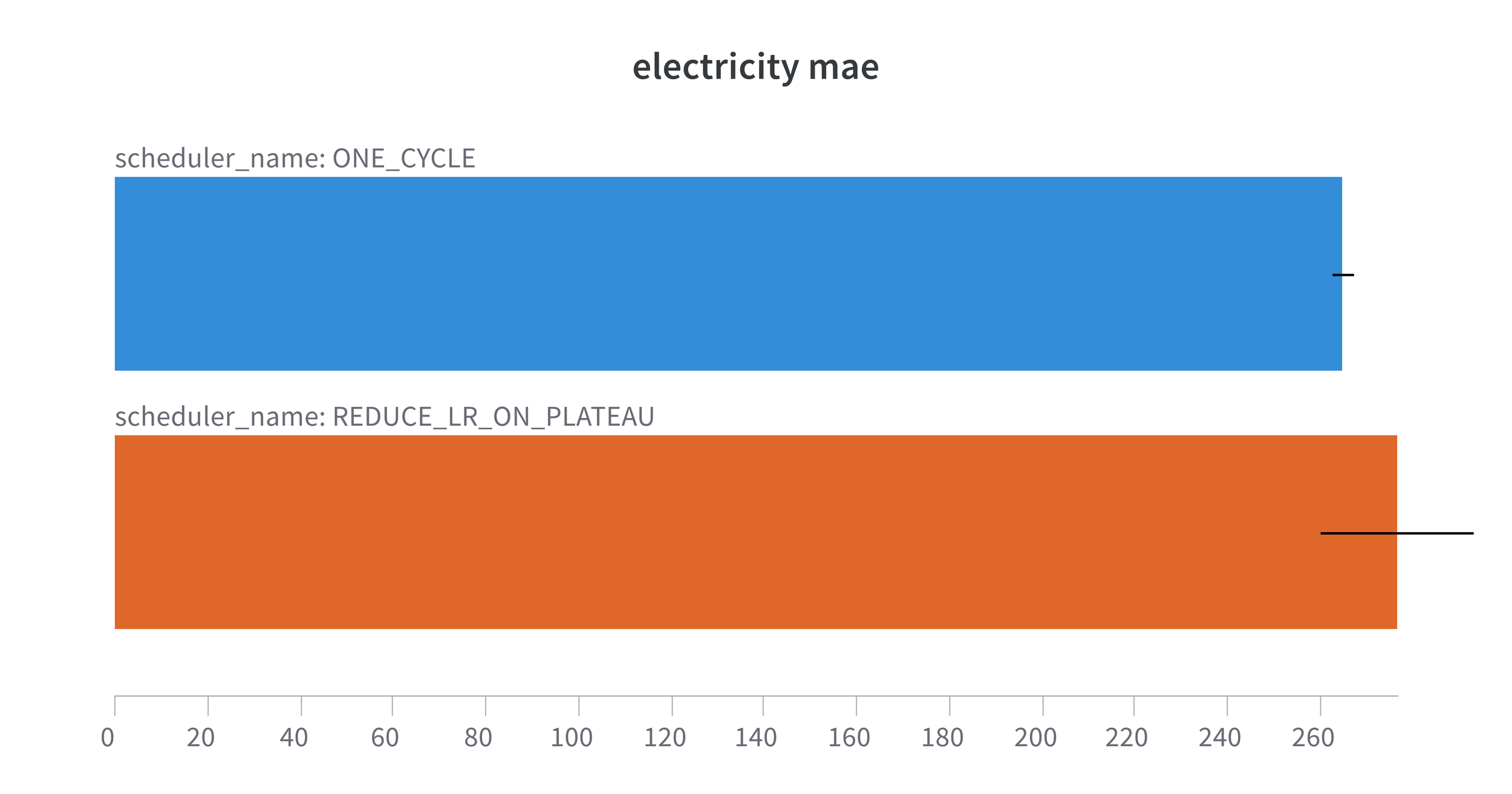
Figure 3. 1Cycle MAE with our model on the Monash Electricity hourly dataset. Forecast Horizon = 168 steps wandb

Figure 4. 1Cycle MAE with our model on the Monash Hospital monthly dataset. Forecast Horizon = 12 steps wandb

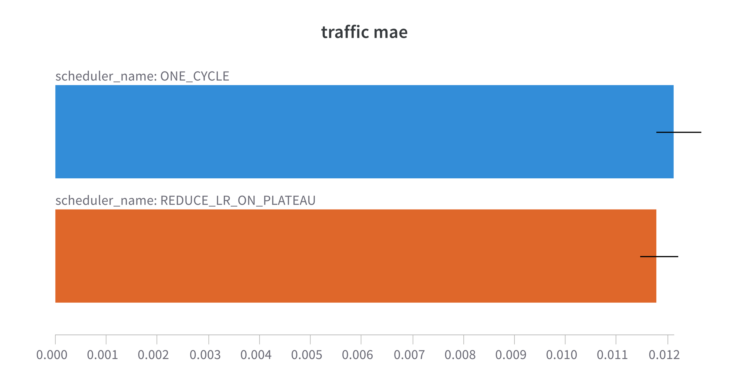
Figure 5. 1Cycle performance with our model on the Monash Traffic hourly dataset. Forecast Horizon = 168 steps wandb

So, here we are looking at the Mean Absolute Error (MAE) for each of the datasets trained with the modified model which contains only lag features and uses a slightly modified scaling function. The results are with my usual 5 runs with different seeds and I am showing both the mean and the error bars are the std error to show the level of variation between the 5 runs. With the exception of Traffic where performance with 1Cycle is marginally inferior to the ReduceLROnPlateau we see an improvement when using 1Cycle. Not only do we see the obvious reduction in MAE when using 1Cycle, but we also see a reduction in the variation between the 5 runs. In other words we are getting more consistent results using 1Cycle. All the results are available on the fantastic wandb platform.

Dataset	Modified DeepAR ReduceLROnPlateau (ours)	Modified DeepAR 1Cycle (ours)	Monash Ranking
Tourism	1.482	1.409	=1 from 13
Electricity	1.628	1.554	1 from 14
Traffic	0.7894	0.809	1 from 14
Hospital	0.7855	0.763	3 from 14

Table 2. Comparison of MASE metrics for our modified DeepAR model with different schedulers

What’s more is that these results start to get quite interesting when we compare them to the Monash set of benchmarks. We see that it is the best performing model on the Electricity, Traffic and Tourism datasets. It is also the third best performing model on the Hospital dataset. So we have managed to improve on the Monash benchmarks with our modified DeepAR model trained with 1Cycle scheduling.

5. Conclusion

So here are come closing thoughts that I have taken from this exercise:

1. 1Cycle scheduling can give a more consistent result that is closer to the optimum than the default ReduceLROnPlateau scheduler.
2. Using covariate features that are not lag variables is not always necessary to get good performance.
3. Using a probabilistic (distribution) appears to trump using a point prediction model.
4. Local scaling matters and the scaling function should be considered carefully for the data that you are working with.

One last thing that I will just mention is that there is a way to improve the point forecast model which puts it on par with the StudentT model, but I will leave that for another post.

All the code for this post can be found on my nnts repo as part of the DeepAR project.